Tag: <span>MapReduce</span>

In this part we will see what Bloom Filters are and how to use them in Hadoop.

We will first focus on creating and testing a Bloom Filter for the Projects dataset. Then we will see how to use that filter in a Repartition Join and in a Replicated Join to see how it can help optimize either performance or memory usage.

Bloom Filter

Hadoop Basics

The Repartition Join we saw in the previous part is a Reduce-Side Join, because the actual joining is done in the reducer. The Replicated Join we are going to discover in this post is a Map-Side Join. The joining is done in mappers, and no reducer is even needed for this operation. So in a sense it should be faster join, but only if certain requirements are met.

We will see how it works and try using it on our Donations/Projects datasets and see if we can accomplish the same join we did in the previous post.

Hadoop Basics

In this part we will see how to perform a Repartition Join in MapReduce. It is also called the Reduce-Side Join because the actual joining of data happens in the reducers. I consider this type of join to be the default and most natural way to join data in MapReduce because :

  • It is a simple use of the MapReduce paradigm, using the joining keys as mapper output keys.
  • It can be used for any type of join (inner, left, right, full outer …).
  • It can join big datasets easily.

Join TypesWe will first create a second dataset, “Projects”, which can be joined to the “Donations” data which we’ve been using since Part I. We will then pose a query that we want to solve. Then we will see how the Repartition Join works and use it to join both datasets and find the result to our query. After that we will see how to optimize our response time.

Hadoop Basics

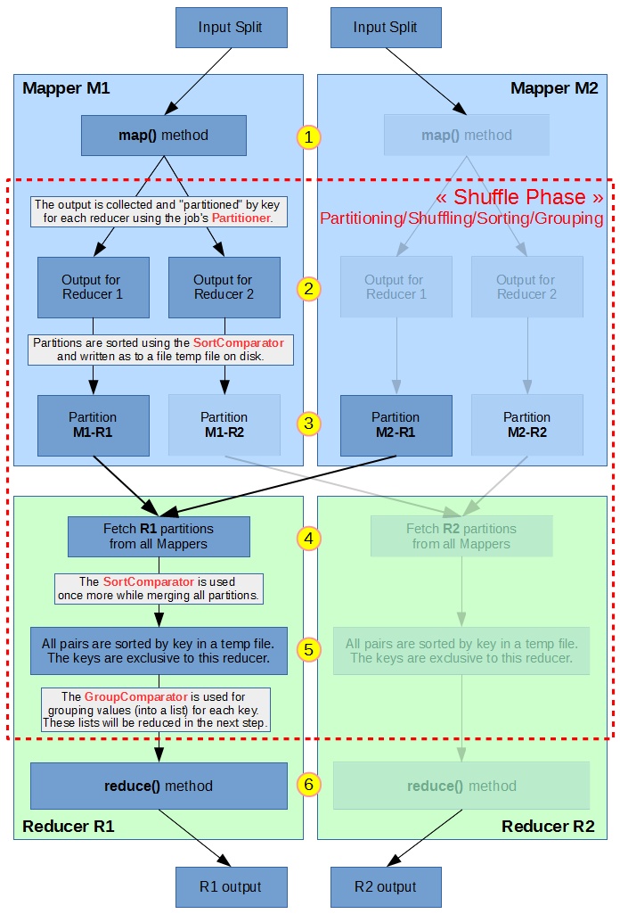
We saw in the previous part that when using multiple reducers, each reducer receives (key,value) pairs assigned to them by the Partitioner. When a reducer receives those pairs they are sorted by key, so generally the output of a reducer is also sorted by key. However, the outputs of different reducers are not ordered between each other, so they cannot be concatenated or read sequentially in the correct order.

For example with 2 reducers, sorting on simple Text keys, you can have :
– Reducer 1 output : (a,5), (d,6), (w,5)
– Reducer 2 output : (b,2), (c,5), (e,7)
The keys are only sorted if you look at each output individually, but if you read one after the other, the ordering is broken.

The objective of Total Order Sorting is to have all outputs sorted across all reducers :
– Reducer 1 output : (a,5), (b,2), (c,5)
– Reducer 2 output : (d,6), (e,7), (w,5)
This way the outputs can be read/searched/concatenated sequentially as a single ordered output.

In this post we will first see how to create a manual total order sorting with a custom partitioner. Then we will learn to use Hadoop’s TotalOrderPartitioner to automatically create partitions on simple type keys. Finally we will see a more advanced technique to use our Secondary Sort’s Composite Key (from the previous post) with this partitioner to achieve “Total Secondary Sorting“.

Hadoop Basics

Shuffle phase workflow

In the previous part we needed to sort our results on a single field. In this post we will learn how to sort data on multiple fields by using Secondary Sort.

We will first pose a query to solve, as we did in the last post, which will require sorting the dataset on multiple fields. Then we will study how the MapReduce shuffle phase works, before implementing our Secondary Sort to obtain the results for the given query.

Hadoop Basics

Now that we have a Sequence File containing our newly “structured” data, let’s see how can get the results to a basic query using MapReduce.

MapReduce SketchWe will illustrate how filtering, aggregation and simple sorting can be achieved in MapReduce. For beginners, these are fundamental operations that can help you understand the MapReduce framework. Advanced readers can still read it quickly to get familiar with the dataset and get ready for the next posts which will be about more advanced sorting and joining techniques.

Hadoop Basics

Benchmark ArtIn this part, we will run a simple Word Count application on the cluster using Hadoop and Spark on various platforms and cluster sizes.

We will run and benchmark the same program on 5 datasets of different sizes on :

  • A single MinnowBoard MAX, using a multi-threaded simple java application
  • A real home computer (my laptop), using the same simple java application
  • MapReduce, using a cluster of 2 to 4 slaves
  • Spark, using a cluster of 2 to 4 slaves

Using these results we will hopefully be able to answer to the original questions of this section : is a home cluster with such small computers worth it ? How many nodes does it take to be faster than a single node, or faster than a real computer ?

Mini-Cluster

Hadoop Spark logos

In this part, we will see how to install and configure Hadoop (2.7.1) and Spark (1.5.1) to have one master and four slaves.

The configurations in this part are adapted for MinnowBoard SBCs. I tried to give as much explanations on the chosen values, which are relative to the resources of this specific cluster. If you have any questions, or if you doubt my configuration, feel free to comment. 🙂

We start by creating a user which we will use for all Hadoop related tasks. Then we will see how to install and configure the master and slaves. Finally we will finish by running a simple MapReduce job to check that everything works and to start being familiar with the Hadoop ecosystem.

Mini-Cluster