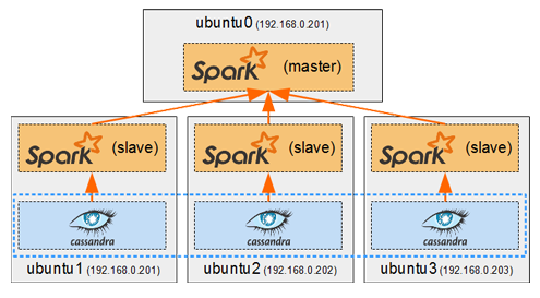
Spark in a general cluster-computing framework, and in our case we will use it to process data from the Cassandra cluster. As we saw in Part I, we cannot run any type of query on a Cassandra table. But by running a Spark worker on each host running a Cassandra node, we can efficiently read/analyse all of its data in a distributed way. Each Spark worker (slave) will read the data from its local Cassandra node and send the result back to the Spark driver (master). 
Nico's Blog Posts
Now that we have deployed containers to have a Cassandra cluster and a Replicated MySQL cluster, it’s time to create the web application which will make use of them. We will create Docker images a proxied Django/uWSGI/Nginx web app, which will connect to the MySQL cluster for OLTP data (django authentication, sessions, etc…), and to the Cassandra cluster for OLAP data (stored user posts).
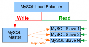
 In the previous part we use the official Cassandra images from Docker Hub to start containers and have them form a cluster. In this post we will see how to create our own docker images to facilitate the deployment of a Master-Slave replicated MySQL cluster. We will also use a HAProxy container to load-balance our MySQL instances.
 In this part we will learn how to run Docker containers. We will explore the basic Docker commands while deploying a small Cassandra cluster on separate hosts on my cluster. To keep things simple we will use the official Cassandra image from Docker Hub to create the Cassandra containers. I will also explain a few basic Cassandra principles and keep it simple for people who have no knowledge of Cassandra.
 In my previous series of posts, I’ve focused on using distributed computing frameworks, Hadoop and Spark, which had to be manually installed on Ubuntu on my cluster nodes.
In this series of posts I will write about how to use Docker to achieve automated distribution-independent deployment of any type of services on my cluster.
 MySQL Master-Slave replication is natively supported by MySQL. However its configuration is not so simple. For each slave added as a replica, a few configuration steps must be done on both the master and itself.
So if you want to install a master instance on a machine or VM, and then install 5 other instances as slaves on other hosts, you will be doing quite a lot of back-and-forth configuration. I couldn’t find any way of configuring the replication automatically on the web, so I decided to create my own bash script to do it.
 In this part, we will use Hive to execute all the queries that we have been processing since the beginning of this series of tutorials.
In nearly all parts, we have coded MapReduce jobs to solve specific types of queries (filtering, aggregation, sorting, joining, etc…). It was a good exercise to understand Hadoop/MapReduce internals and some distributed processing theory, but it required to write a lot of code. Hive can translate SQL queries into MapReduce jobs to get results of a query without needing to write any code.
We will start by installing Hive and setting up tables for our datasets, before executing our queries from previous parts and seeing if Hive can have better execution times than our hand-coded MapReduce jobs.
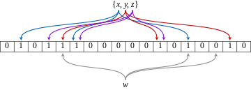
In this part we will see what Bloom Filters are and how to use them in Hadoop.
We will first focus on creating and testing a Bloom Filter for the Projects dataset. Then we will see how to use that filter in a Repartition Join and in a Replicated Join to see how it can help optimize either performance or memory usage.
The Repartition Join we saw in the previous part is a Reduce-Side Join, because the actual joining is done in the reducer. The Replicated Join we are going to discover in this post is a Map-Side Join. The joining is done in mappers, and no reducer is even needed for this operation. So in a sense it should be faster join, but only if certain requirements are met.
We will see how it works and try using it on our Donations/Projects datasets and see if we can accomplish the same join we did in the previous post.
In this part we will see how to perform a Repartition Join in MapReduce. It is also called the Reduce-Side Join because the actual joining of data happens in the reducers. I consider this type of join to be the default and most natural way to join data in MapReduce because :
- It is a simple use of the MapReduce paradigm, using the joining keys as mapper output keys.
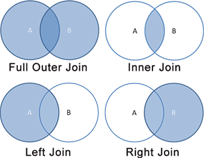
- It can be used for any type of join (inner, left, right, full outer …).
- It can join big datasets easily.
 We will first create a second dataset, “Projects”, which can be joined to the “Donations” data which we’ve been using since Part I. We will then pose a query that we want to solve. Then we will see how the Repartition Join works and use it to join both datasets and find the result to our query. After that we will see how to optimize our response time.

