In this part we will see what Bloom Filters are and how to use them in Hadoop.
We will first focus on creating and testing a Bloom Filter for the Projects dataset. Then we will see how to use that filter in a Repartition Join and in a Replicated Join to see how it can help optimize either performance or memory usage.
Contents
Bloom Filters
Introduction
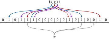
A Bloom Filter is a space-efficient probabilistic data structure that is used for membership testing.
To keep it simple, its main usage is to “remember” which keys were given to it. For example you can add the keys “banana”, “apple” and “lemon” to a newly created Bloom Filter. And then later on, if you ask it whether it contains “banana” it should reply true, but if you ask it for “pineapple” it should reply false.
A Bloom Filter is space-efficient, meaning that it needs very little memory to remember what you gave it. Actually it has a fixed size, so you even get to decide how much memory you want it to use, independently of how many keys you will pass to it later. Of course this comes at a certain cost, which is the possibility of having false positives. But there can never be false negatives. This means that in our fruity example, if you ask it for “banana” it has to reply true. But is you ask it for “pineapple”, there is a small chance that it might reply true instead of false.
Theory and False Positive Estimation
For detailed explanations on how Bloom Filters work, you can read this wikipedia page.
I will only explain here what are the characteristics and how to use them in a simple calculation to estimate the false positive rate.
Let’s consider a Bloom filter with the following characteristics:
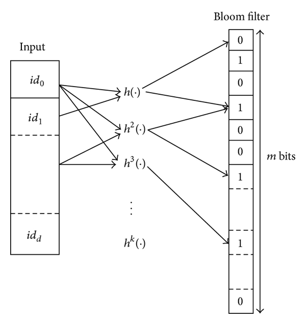
- m : number of bits in the array
- k : number of hash functions
- n : number of keys added for membership testing
- p : false positive rate (probability between 0 and 1)
The relation between theses values can be expressed as :
££\begin{aligned}
\\[5pt]m & = -\frac{n\,ln (p)}{ln(2)^2} & (1)
\\[5pt]k & = \frac{m}{n} ln(2) & (2)
\\[5pt]p & \approx (1 – e^{-\frac{k\,n}{m}})^k & (3)
\end{aligned}££
Let’s create a filter which will contain all Project ids where the subject is about science, while aiming for a 1% false positive rate. Here are the steps on how to do this.
Step 1: Estimate the number of entries which will added
By doing a “grep” on the first 100 lines of the original csv dataset, I found out that a bit less than 20 rows contain the word “science” in their subject. So we can consider than approximately 20% of all records have a subject about science.
There are around 880k records in the dataset. Let’s round that up to 1 million.
The number of entries which will be added to the filter should be less than 20% of 1 million, n = 200,000.
Step 2: Calculate the number of bits to use in the array
Using formula (1), with p=0.01 for 1% false positive rate :
££ m = -\frac{200{,}000\,ln (0.01)}{ln(2)^2} = 1,917,011
\\[18pt] m \approx\,2{,}000{,}000\,bits ££
Step 3: Calculate the number of hash functions
Using formula (2):
££ k = \frac{2{,}000{,}000}{200{,}000} ln(2) = 6.93
\\[18pt] k = 7\, hashes ££
Step 4: Verify the False Positive Rate
We can now re-evaluate our FP rate, using formula (3):
££ p \approx (1 – e^{-\frac{7*200{,}000}{2{,}000{,}000}})^7 \approx 0.00819
\\[8pt] p \approx 0.8\% ££
So around 0.8% of all entries which do not contain the word “science” in their subject will still show up as containing “science” when using a filter with these characteristics. But only if 200,000 entries are added to it. If in practice less entries are added, the error rate would decrease. And if more entries were added, the error rate would get worse.
If the False Positive Rate (FPR) you end up with seems too high, you can go back to Step 2 and use a smaller value of p. If you are unsure of the number of keys and are scared to be unlucky and get a higher FPR, choose an over-estimated value of n.
Creating the filter in Hadoop
Here is a MapReduce job which creates the exact same filter that we described in the previous paragraph: https://github.com/nicomak/[…]/ProjectBloomFilter.java
All instances of BloomFilter in this job are created using the values of m and k we agreed on in the previous paragraph:
BloomFilter filter = new BloomFilter(2_000_000, 7, Hash.MURMUR_HASH);
Each mapper goes through its own projects.seqfile input split. Whenever the condition is satisfied on a record (when the subject contains “science”), it adds the record’s ID to its own BloomFilter instance, using the BloomFilter.add(Key key) method.
Each mapper will wait for all records to be processed, before writing the BloomFilter writable object to its output. It does this inside the cleanup() method, only after all map() method calls have been completed.
Then a single reducer is used to receive all Bloom Filters from all mappers, and merge them by logical OR into its own instance of BloomFilter, using the BloomFilter.or(Filter filter) method. In the cleanup() method, the reducer writes the final merged Bloom Filter to a file in HDFS.
Job execution console:
$ hadoop jar donors.jar mapreduce.join.bloomfilter.ProjectBloomFilter donors/projects.seqfile donors/projects_science_bloom

$ hdfs dfs -ls -h donors/projects_science_bloom
Found 1 items
-rw-r--r--   2 hduser supergroup    244.2 K 2016-02-05 12:22 donors/projects_science_bloom/filter
The MapReduce job takes around 1 min 30 s on my mini-cluster.
It automatically creates a file called “filter” in the given destination folder. We can see that the file is quite small, and corresponds roughly to the size of our 2,000,000 bits array. According to the log I added in the cleanup method, there were 123,099 keys inserted in the filter. That’s significantly less than the 200k we estimated, which means that our error rate should be also less than the 0.8% we were expecting. Let’s check this out while testing our filter.
Testing the filter in Hadoop
Now we will run a job which goes through all records of the projects.seqfile data and check if their subjects contain “science” with both tests:
- a : Testing the ID membership in the Bloom Filter we just created
- b : Doing the string search again
For each record, it will print out the following :
| Case | Output |
| a == b | (nothing) |
| a && !b | FALSE_POSITIVE: <project_id> |
| !a && b | FALSE_NEGATIVE: <project_id> |
This will help us confirm that there are no False Negatives, and let us count how many false positives were given by our filter.
The MapReduce job is here: https://github.com/nicomak/[…]/ProjectFilterTest.java
$ hadoop jar donors.jar mapreduce.join.bloomfilter.ProjectFilterTest donors/projects.seqfile donors/projects_science_bloom/filter donors/output_filter_test

$ hdfs dfs -ls -h donors/output_filter_test
Found 2 items
-rw-r--r--   2 hduser supergroup          0 2016-02-05 13:09 donors/output_filter_test/_SUCCESS
-rw-r--r--   2 hduser supergroup     21.8 K 2016-02-05 13:09 donors/output_filter_test/part-m-00000

hdfs dfs -cat donors/output_filter_test/part-m-00000
FALSE_POSITIVE  a09925c883a884e6289c27a6ce5f792e
FALSE_POSITIVE  b0a3948ef06a84975ee942f36a25be08
FALSE_POSITIVE  3afc91503e89f8da24b56554d5830862
FALSE_POSITIVE  66d75fb0848f9cf3161b0a47b3f0c51b
...
FALSE_POSITIVE  aae635504a700bc6a1c1a49dad4a3e2e
FALSE_POSITIVE  33a3cb0d623c5f56ac219aa5b51ef7e3
FALSE_POSITIVE  7fae9e1a8cedbb8bfde78a1e68281d99
FALSE_POSITIVE  75f7b83e93d0181732b4624df8ea9492

hdfs dfs -cat donors/output_filter_test/part-m-00000 | wc -l
466
Well, as excepted there were no false negatives. And there were 466 false positives, for a total of 123,009 keys.
Let’s calculate the theoretical false positive rate, and compare it to the real false positive rate observed during this test.
In theory, according to formula (3):
££ p \approx (1 – e^{-\frac{7*123{,}099}{2{,}000{,}000}})^7 \approx 0.0006439
\\[8pt] p \approx 0.064\% ££
The real false positive rate can be calculated by:
££ fpr = \frac{False Positives}{Negatives} = \frac{123{,}099}{878{,}853-123{,}099} = 0.000617
\\[18pt] fpr \approx 0.062\% ££
The theoretical and real value are very close ! And they are both a lost smaller than the original false positive rate of 0.8% estimated when we thought we would have as much as 200,000 keys satisfying the filter condition.
Creating a filter without any false positives
If you cannot accept any false positive in your use-case, you have to play with the variables again and decrease the error rate enough to make FPs disappear.
Using an array size of 10 million bits instead of 2 million bits, our FPR becomes:
££ p \approx (1 – e^{-\frac{7*123{,}099}{10{,}000{,}000}})^7 \approx 0.000000026
\\[8pt] p \approx 0.0000026\% ££
With this theoretical error rate, we should have approximately p * Negatives = 0.000000026*755754 = 0.02 FP occurrences in the whole dataset.
This means that we are very likely to have no FP at all, and to have a perfect filter.
Using 10 million bits for all filters in both mapreduce jobs (creation and testing), the size of the filter in HDFS is 1.19 MB, and the testing output file is empty, meaning that there are no false positives.
This filter is 100% accurate and we will now use it to optimize our joins from the previous posts.
Optimizing Joins
In the previous 2 posts which discussed the Repartition Join and the Replicated Join techniques, we joined full datasets without filtering data on either side.
When the query has conditions on the datasets to be joined, using a Bloom Filter can be very useful.
Repartition Join
This time we will slightly change our join query to add a condition on the Projects dataset. We will only keep Projects whose subjects are about Science:
SELECT d.donation_id, d.project_id as join_fk, d.donor_city, d.ddate, d.total, p.project_id, p.school_city, p.poverty_level, p.primary_focus_subject
FROM donations as d
INNER JOIN projects as p
ON d.project_id = p.project_id
WHERE LOWER(p.primary_focus_subject) LIKE '%science%';
We can process this query using a Repartition Join by simply discarding all projects which do not contain the word “science” in their subject in the ProjectsMapper.
The code for this basic repartition join can be viewed here on GitHub, and takes around 2 min 45 s on my cluster.
We can optimize this execution time my using the Bloom Filter we created in the previous section. What is really interesting is that this filter was meant to filter out Projects, but we can also use it to filter out Donations. In the DonationsMapper, we can apply the Bloom Filter on the “donation.project_id” joining key and skip records for which the filter replies false. This will discard all Donations which would have been joined to projects not satisfying the condition.
Using the Bloom Filter can help cut down useless data from both sides of the join even before the shuffle phase, making all mappers faster.
The code for this can be viewed here: https://github.com/nicomak/[…]/RepartitionJoinScienceProjectsBloom.java
The job took only 2 min 00 sec on average when using the Bloom Filter.
Replicated Join
The Inner Join query can also be processed using a Replicated Join. We can discard all projects which do not contain the word “science” before they enter the cache map which is used for joining in each Mapper.
The code for this basic replicated join can be viewed here on GitHub. It took 1 min 48 sec on average on my mini-cluster. This is already quite fast and we won’t make it faster by using a Bloom Filter.
But the problem of Replicated Joins is not speed. The problem is often that the right-side dataset cannot fit into memory.
In the previous part, I said that if a dataset can’t fit into the mapper’s RAM, we can use a Semi-Join to pre-eliminate all useless right-side records (based on both sides conditions) before the real join job. In step 2 of that process, a Replicated join must be performed between the right-side dataset (read from HDFS input splits) and the cached text list of pre-generated IDs of records satisfying the query conditions.
However, it may be possible, when using huge datasets, that even a list of IDs does not fit into memory. If your list of 32-character IDs contains 1 billion entries, it will need around 100 GB of memory in Java to store them in your cache. In that case you can use a Bloom Filter for your 1 billion keys. Using formula (3) again, with still 7 hash functions, if we use 10 billion bits as the array size, we keep the False Positive rate under 1%.
That would take a bit more than 1 GB of memory only instead of 100 GB, and would maximize its chances of fitting into memory.
interesting algorithm using hash.
thanks for sharing